Preliminary Result of the Apr 11, 2012 Mw 8.64 sumatra Earthquake
Guangfu Shao, Xiangyu Li, Chen Ji, UCSB
DATA Process and Inversion
We used the GSN broadband waveforms downloaded from the IRIS DMC. We analyzed 28 teleseismic broadband P waveforms, 27 broadband SH waveforms, and 45 long period surface waves selected based upon data quality and azimuthal distribution. Waveforms are first converted to displacement by removing the instrument response and then used to constrain the slip history based on a finite fault inverse algorithm (Ji et al, 2002). We use the hypocenter of the USGS (Lon.=93.0600 deg.; Lat.=2.3100 deg.). The fault planes are defined using the quick moment tensor solution of the Global.
Result
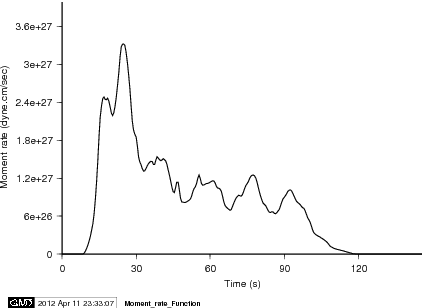
After comparing the waveform fits based on two planes, we find that the nodal plane (strike=20.00 deg., dip=80.00 deg.) fits the data better. The seismic moment release based upon this plane is
0.117E+30 dyne.cm using a 1D crustal model interpolated from CRUST2.0 (Bassin et al., 2000).
Cross-section of slip distribution
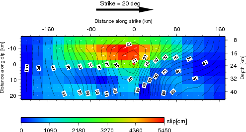
Figure 1.1 Cross-section of slip distribution. the strike direction of fault plane is indicated by the black arrow and the hypocenter location is denoted by the red star. The slip amplitude are showed in color and motion direction of the hanging wall relative to the footwall is indicated by white arrows. Contours show the rupture initiation time in seconds.
Moment rate function
Comparison of data and synthetic seismograms
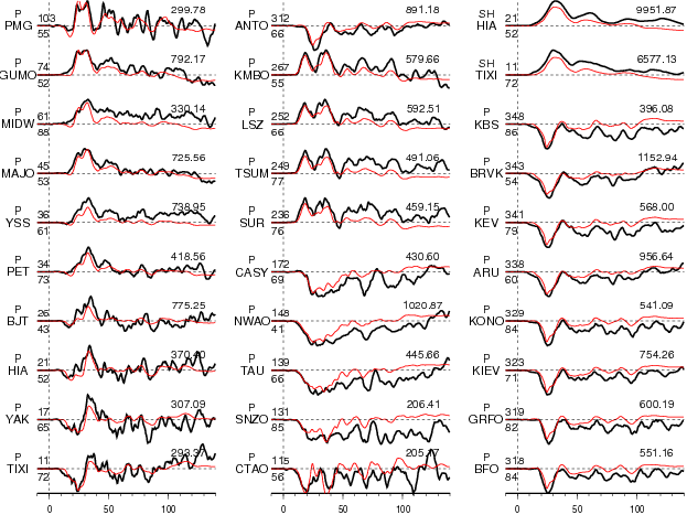
Figure 2.1. Comparison of teleseismic body waves. The data is shown in black and the synthetic seismograms are plotted in red. Both data and synthetic seismograms are aligned on the P or SH arrivals. The number at the end of each trace is the peak amplitude of the observation in micro-meter. The number above the beginning of each trace is the source azimuth and below is the epicentral distance.
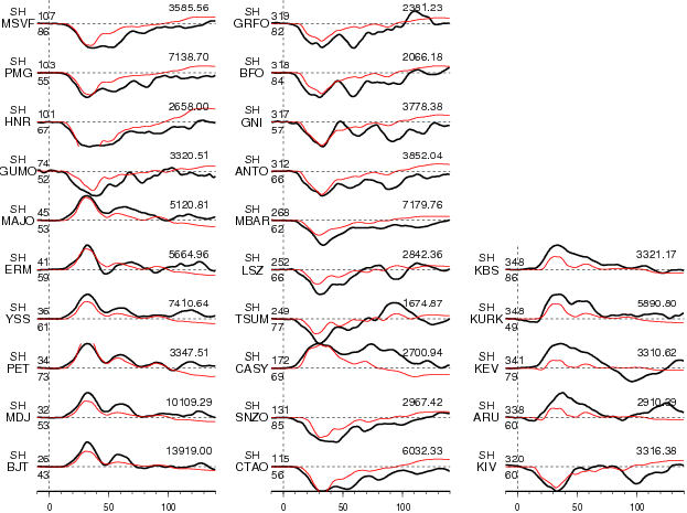
Figure 2.2. Comparison of teleseismic body waves. The data is shown in black and the synthetic seismograms are plotted in red. Both data and synthetic seismograms are aligned on the P or SH arrivals. The number at the end of each trace is the peak amplitude of the observation in micro-meter. The number above the beginning of each trace is the source azimuth and below is the epicentral distance.
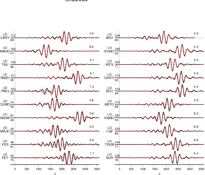
Figure 3.1. Comparison of long period surface waves. The data is shown in black and the synthetic seismograms are plotted in red. Both data and synthetic seismograms are aligned on the P or SH arrivals. The number at the end of each trace is the peak amplitude of the observation in micro-meter. The number above the beginning of each trace is the source azimuth and below is the epicentral distance.
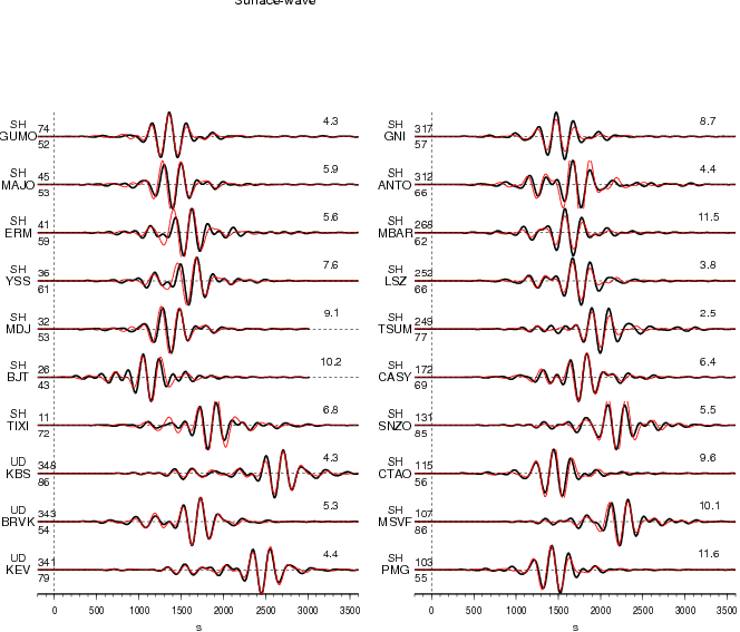
Figure 3.2. Comparison of long period surface waves. The data is shown in black and the synthetic seismograms are plotted in red. Both data and synthetic seismograms are aligned on the P or SH arrivals. The number at the end of each trace is the peak amplitude of the observation in micro-meter. The number above the beginning of each trace is the source azimuth and below is the epicentral distance.
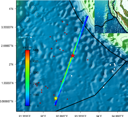
Figure 4. Surface projection of the slip distribution superimposed on ETOPO2. The black line indicates the major plate boundary [Bird, 2003]. The white dots are background seismicity from 1964 to 2004 (Relocated ISC catalog, Engdahl et al, 1998). The red dots are aftershocks in a day(NEIC USGS). Yellow star denotes the epicenter of the M8.2 aftershock.
CJ's Comments:
1. Fault Plane
The waveform fits, particularly the fits to P waves, suggest that the N-S oriented plane is better than the E-W plane. Of course, such a conclusion depends on the precision of focal mechanism and Green's functions.
If we choose E-W fault plane (strike 110 or 290 degrees), the focal mechanisms of GCMT, USGS W-phase, USGS traditional CMT all suggest that it has a nearly vertical fault plane. If this is held, we cannot fit the P-wave waveforms at SUR, TSUM, LSZ, KMBO (their azimuths change from 236 to 267 degrees). They have double pulses in the first 40 s. In contrast, the waveforms at stations on other side of plane, ANTO, BFO, GRFO etc, (azimuths changing from 312 to 340 degrees), feature a single-pulse. In a restricted sense, this argument is held for the first 40 s.
A preliminary slip model using the E-W fault plane done by Dr. Hayes can be found at the USGS Website.
2. Rupture duration
We have noticed the existence of second subevent which initiated at about 200 s. However, its seismic moment is much smaller than the first one and we have not obtained a stable solution yet.
Slip Distribution
References
Ji, C., D.J. Wald, and D.V. Helmberger, Source description of the 1999 Hector Mine, California earthquake; Part I: Wavelet domain inversion theory and resolution analysis, Bull. Seism. Soc. Am., Vol 92, No. 4. pp. 1192-1207, 2002.
Bassin, C., Laske, G. and Masters, G., The Current Limits of Resolution for Surface Wave Tomography in North America, EOS Trans AGU, 81, F897, 2000.
Acknowledgement and Contact Information
This work is supported by National Earthquake Information Center (NEIC) of United States Geological Survey. This web page is built and maintained by Dr. C. Ji at UCSB.