Rupture process of the 2007 April 1 Magnitude 8.1 - Solomon Islands Earthquake
Chen Ji, UCSB
DATA Process and Inversion
We selected 17 teleseismic P and 16 SH body waveforms, which were first converted to displacement by removing the instrument response and then bandpass filtered from 2 sec to 330 sec. The time window used in this study is about 160 sec. We also included 15 long period Rayleigh waves and 12 long period Love waves into inversions. We defined the fault plane using the hypocenter location of the USGS (Lat.=-8.45 deg.; Lon.=156.96 deg. ), the moment tensor solution of the Quick CMT (Dr. Polet), and trench axis. We constrained its rupture process using a finite fault inverse algorithm in wavelet domain (Ji et al, 2002, 2003).
Result
We selected the low angle nodal plane (dip =25 deg., strike=305 deg.) as preferred fault plane based upon aftershock distribution. Its dimension is 300 km (along strike) by 90 km, which is further divided into 180 subfaults (15 km by 10 km). The seismic moment release of this model is 1.8x10²¹ N.m and its peak slip is about 4 m using the Crust2.0 Model.
Cross-section of slip distribution
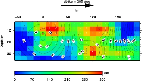
Caption: A big black arrow indicates the strike of the fault plane. The color
shows the amplitude of dislocations and white arrows represent the motion of
the hanging wall relative to the footwall. Contours show the rupture initiation
time in sec and the red star indicates the hypocenter location.
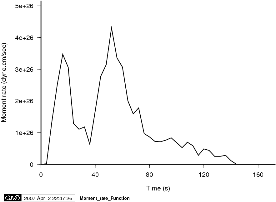
Caption: Moment rate function.
Comparison of data and synthetic seismograms
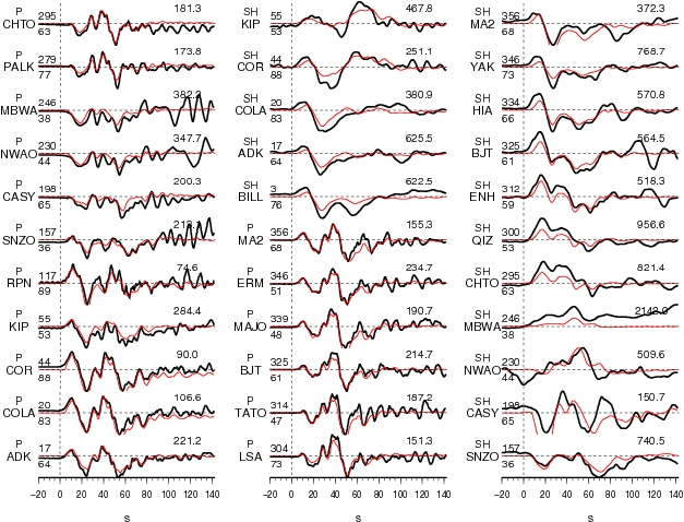
Caption: The Data are shown in black and the synthetic seismograms are plotted
in red. Both of them are aligned on the P or SH arrivals. The number at the end
of each trace is the peak amplitude of the observation in micro-meter. The
number above the beginning of each trace is the azimuth and that below is the
epicentral distance.
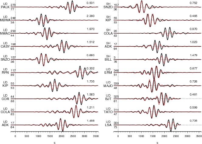
Caption: Comparison of long period Rayleigh (UD) and Love (SH) waves (3 mHz to
6 mHz). The number at the end of each trace is the peak amplitude of the
observation in millimeter.
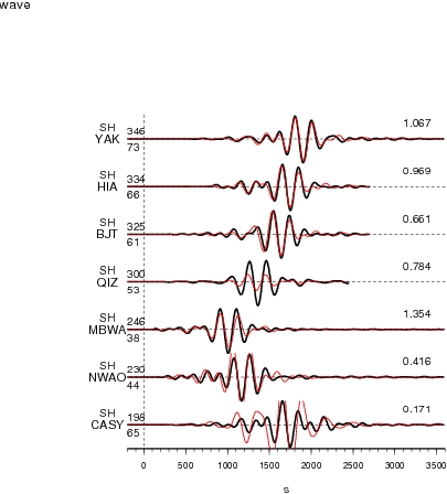
Figure: Comparison of long period Rayleigh (UD) or Love (SH) waves (3 mHz to
6 mHz). The number at the end of each trace is the peak amplitude of the
observation in millimeter.
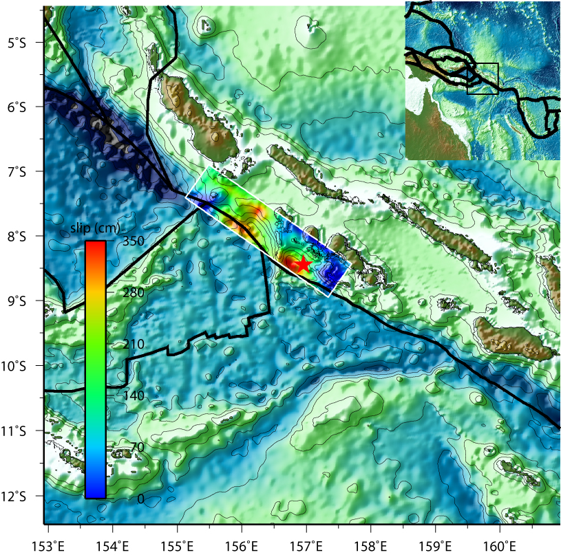
Figure: Surface projection of the slip distribution superimposed on topography
and bathymetric map ETOPO2.
CJ's Comments:
Download (Slip Distribution)
| COULOMB INPUT FORMAT |
CMTSOLUTION FORMAT |
References
Ji, C., D.J. Wald, and D.V. Helmberger, Source description of the 1999
Hector Mine,
Bassin, C., Laske, G. and Masters, G., The Current Limits of Resolution for
Surface Wave Tomography in North America, EOS Trans AGU, 81, F897, 2000.
Acknowledgement and Contact Information
This work is supported by