Rupture process of the 2007 Jan 13
Magnitude 8.1 - KURIL Island Earthquake (Revised)
Chen Ji, UCSB
DATA Process and Inversion
We used the GSN broadband data downloaded from the IRIS DMC
(http://www.iris.washington.edu/). We selected 21 teleseismic P and
17 SH body waveforms, which were first converted to displacement by
removing the instrument response and then bandpass filtered from 2
sec to 330 sec. The time window used in this study is about 160 sec.
We also included 20 long period Rayleigh waves and 19 long period
Love waves into inversions. We defined the fault plane using the
hypocenter location of the USGS (Lat.=46.29 deg.; Lon.=154.45 deg.
Depth = 10 km) and the moment tensor solution of the GLOABL CMT
(http://www.globalcmt.org) after
evaluating them with very long period seismic waves.
The hypocenter depth has been shifted (18 km) to
match the body waves. We constrained its rupture process
using a finite fault inverse algorithm in wavelet domain (Ji et al,
2002, 2003).
Result
We selected the high angle nodal plane (dip =57.89 deg., strike=42
deg.) as preferred fault plane based upon aftershock distribution. Its
dimension is 200 km (along strike) by 35 km, which is further
divided into 175 subfaults (8 km by 5 km). The seismic
moment release of this model is 1.9x10²¹ N.m and its peak slip
is about 20 m using a 1D PREM model.
Cross-section of slip distribution
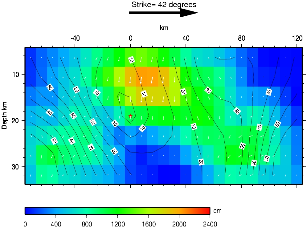
Caption:
A big black arrow indicates the strike of the fault plane. The color
shows the amplitude of dislocations and white arrows represent the
motion of the hanging wall relative to the footwall. Contours show
the rupture initiation time in sec and the red star indicates the
hypocenter location.
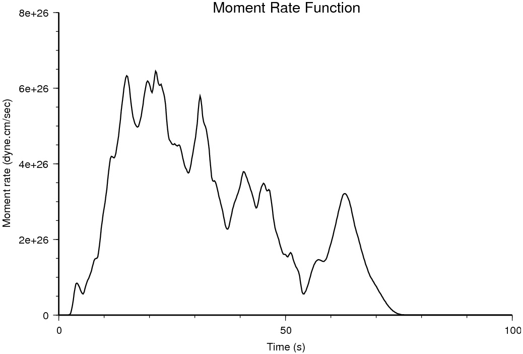
Caption:
Moment rate function.
Comparison of data and synthetic seismograms
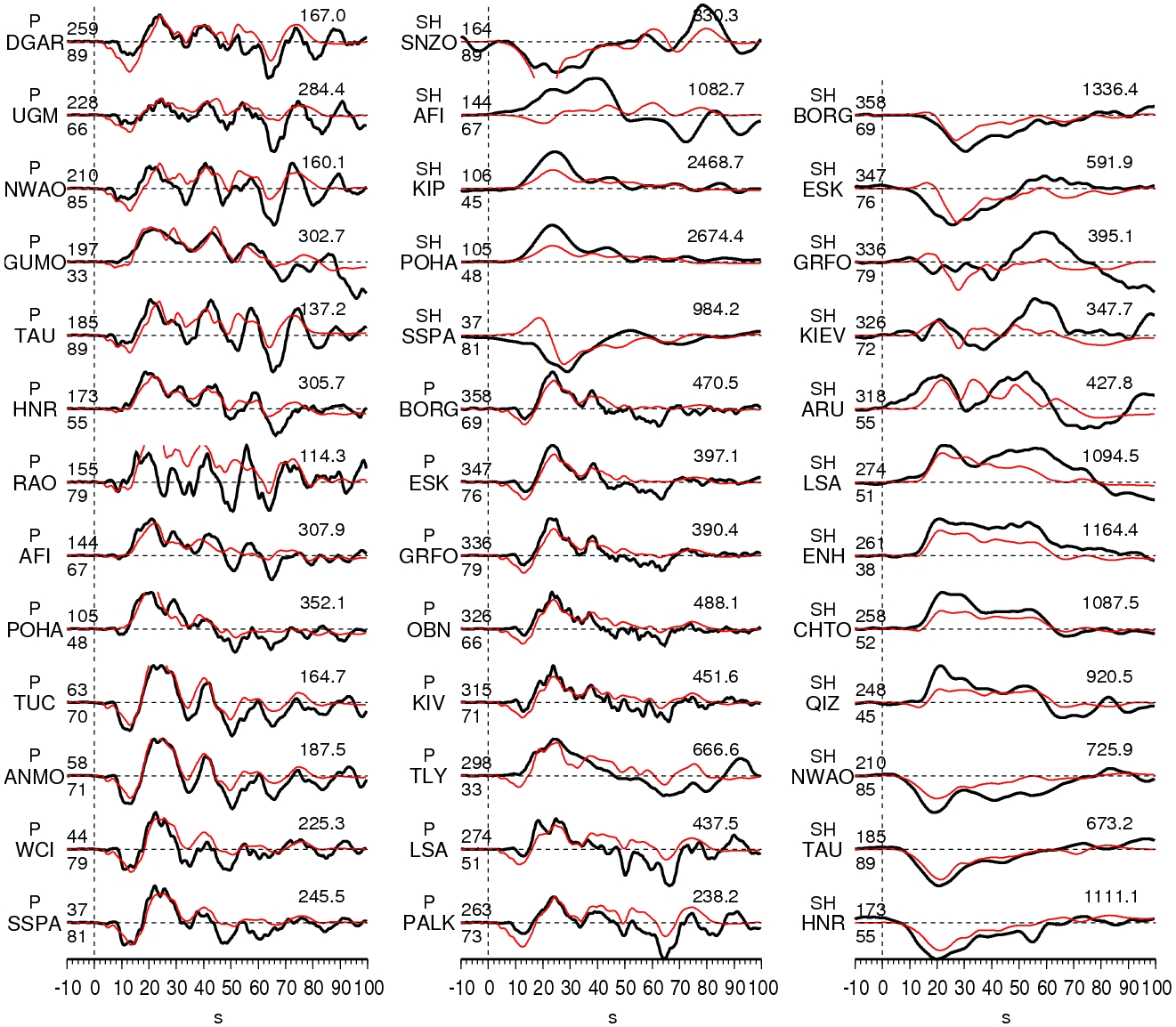
Caption:
The Data are shown in black and the synthetic seismograms are plotted
in red. Both of them are aligned on the P or SH arrivals. The number
at the end of each trace is the peak amplitude of the observation in
micro-meter. The number above the beginning of each trace is the
source azimuth and below is the epicentral distance.
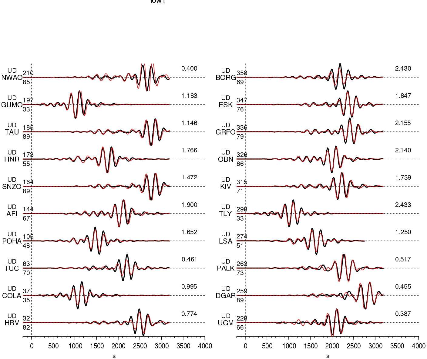
Caption:
Comparison of long period Rayleigh (UD) and Love (SH) waves (30 mHz
to 60 mHz). The number at the end of each trace is the peak amplitude
of the observation in millimeter.
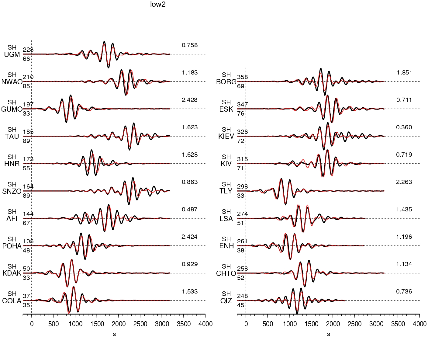
Figure:
Comparison of long period Rayleigh (UD) or Love (SH) waves (30 mHz to
60 mHz). The number at the end of each trace is the peak amplitude of
the observation in millimeter.
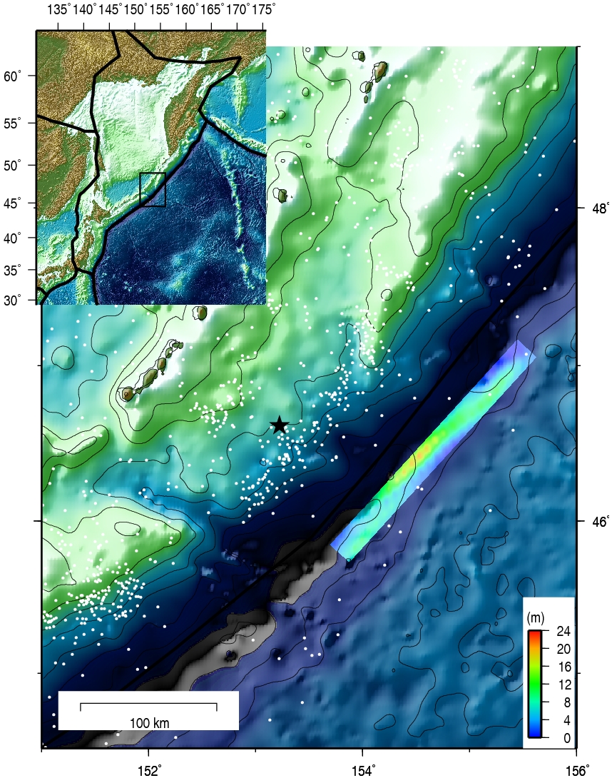
Figure:
Surface projection of the slip distribution superimposed on
topography and bathymetric map ETOPO2. The red contours shows the
slip distribution. The black line indicates the plate boundary. The
white dots are background seismicity from 1964 to 2004 (Relocated ISC
catalog, Engdahl et al, 1998).
CJ's Comments:
I test the focal mechanisms following the trench axis but with smaller dip angles. It could explain the body waves fairly well but fail
to simultanouesly explain the long period Love waves.
Download (Slip Distribution)
References
Ji, C., D.J. Wald, and D.V. Helmberger, Source description of the
1999 Hector Mine, California earthquake; Part I: Wavelet domain
inversion theory and resolution analysis, Bull. Seism. Soc. Am., Vol
92, No. 4. pp. 1192-1207, 2002.
Bassin, C., Laske, G. and
Masters, G., The Current Limits of Resolution for Surface Wave
Tomography in North America, EOS Trans AGU, 81, F897, 2000.
Acknowledgement and Contact Information
This work is supported by National Earthquake Information Center
(NEIC) of United States Geological Survey. This web page is built and
maintained by Dr. C. Ji at
UCSB.