Preliminary Result of the Aug 23, 2011 Mw 5.77 Virginia Earthquake
Guangfu Shao, Chen Ji, UCSB
DATA Process and Inversion
We used the GSN broadband waveforms downloaded from the IRIS DMC. We analyzed 43 teleseismic broadband P waveforms and 22 broadband SH waveforms selected based upon data quality and azimuthal distribution. Waveforms are first converted to velocity by removing the instrument response and then resampled at an interval of 0.05 s. Signals from 12.8 s to 0.5 s for P waves and from 12.8 s to 1 s for SH waves are used to constrain the slip history based on a finite fault inverse algorithm (Ji et al, 2002). We use the hypocenter of the USGS (Lon.=-77.933 deg.; Lat.=37.936 deg.; Depth=5km). The fault planes are defined using the quick moment tensor solution of the NEIC.
Result
We performed two inversions with the two possible fault planes, which are referred from the two nodal planes of the SLU regional moment tensor solutions (nodal plane 1: strike=177 deg., dip=39 deg., rake=66 deg.; nodal plane 2: 26 deg., 55 deg., 119 deg.). We named the inverted results as Model I and Model II, respectively. The fault plane size is 10 km (along strike) by 8 km (along dip) for the Model I and 9 km by 9 km for the Model II. These fault planes are further discretized into 1 km by 1 km subfaults. Totally, there are 80 subfaults for Model I and 81 subfaults for Model II. The total seismic moment is constrained using the Harvard CMT solution. The inverted value is 0.575E+25 dyne.cm for Model I and 0.578E+25 dyne.cm for Model II using a 1D crustal model interpolated from CRUST2.0 (Bassin et al., 2000).
Average stress drop
We estimated the stress drop of the Virginia earthquake using the empirical relationship given by Cohn et al. (1982).
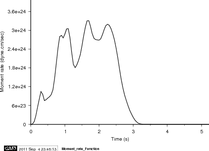
The estimated stress drop is 4 MPa for a total seismic moment of 5.75E+17 N.m and a source duration of 3 s, based on our inversion results (see below).
1. Model I
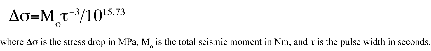
Cross-section of slip distribution
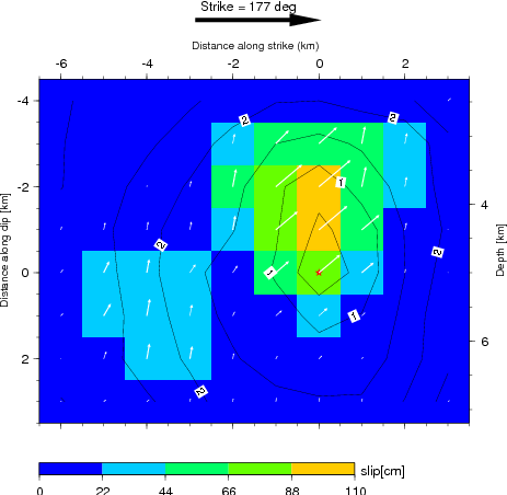
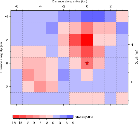
Figure 1.1 Left: Cross-section of slip distribution. The strike direction of fault plane is indicated by the black arrow and the hypocenter location is denoted by the red star. The slip amplitude are showed in color and motion direction of the hanging wall relative to the footwall is indicated by white arrows. Contours show the rupture initiation time in seconds. Right: On-fault stress drop for the motion in the average rake angle direction (60 degrees) calculated from the Model I slip model (left) using the software Coulomb3.2. The average stress drop is 6.0 MPa.
Moment rate function
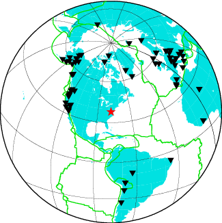
Station distribution
Comparison of data and synthetic seismograms
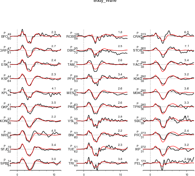
Figure 2.1. Comparison of teleseismic body waves in velocity. The data is shown in black and the synthetic seismograms are plotted in red. Both data and synthetic seismograms are aligned on the P or SH arrivals. The number at the end of each trace is the peak amplitude of the observation in micro-meter per second. The number above the beginning of each trace is the source azimuth and below is the epicentral distance.
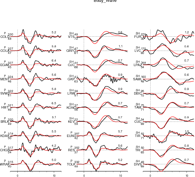
Figure 2.2. Comparison of teleseismic body waves in velocity. The data is shown in black and the synthetic seismograms are plotted in red. Both data and synthetic seismograms are aligned on the P or SH arrivals. The number at the end of each trace is the peak amplitude of the observation in micro-meter per second. The number above the beginning of each trace is the source azimuth and below is the epicentral distance.
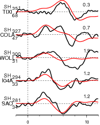
Figure 2.3. Comparison of teleseismic body waves in velocity. The data is shown in black and the synthetic seismograms are plotted in red. Both data and synthetic seismograms are aligned on the P or SH arrivals. The number at the end of each trace is the peak amplitude of the observation in micro-meter per second. The number above the beginning of each trace is the source azimuth and below is the epicentral distance.
Slip Distribution
2. Model II
Cross-section of slip distribution
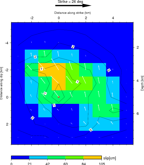
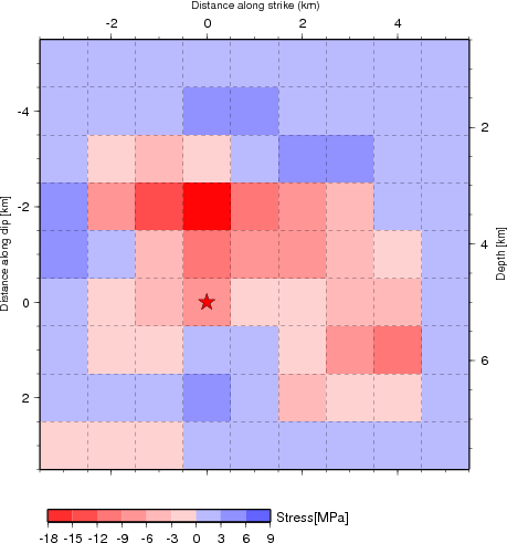
Figure 1.1 Cross-section of slip distribution of Model II. The strike direction of fault plane is indicated by the black arrow and the hypocenter location is denoted by the red star. The slip amplitude are showed in color and motion direction of the hanging wall relative to the footwall is indicated by white arrows. Contours show the rupture initiation time in seconds. Right: On-fault stress drop for the motion in the average rake angle direction (116 degrees) calculated from the Model II slip model (left) using the software Coulomb3.2. The average stress drop is 6.1 MPa.
Moment rate function
Comparison of data and synthetic seismograms
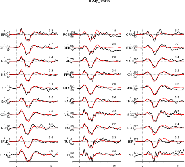
Figure 2.1. Comparison of teleseismic body waves in velocity. The data is shown in black and the synthetic seismograms are plotted in red. Both data and synthetic seismograms are aligned on the P or SH arrivals. The number at the end of each trace is the peak amplitude of the observation in micro-meter per second. The number above the beginning of each trace is the source azimuth and below is the epicentral distance.
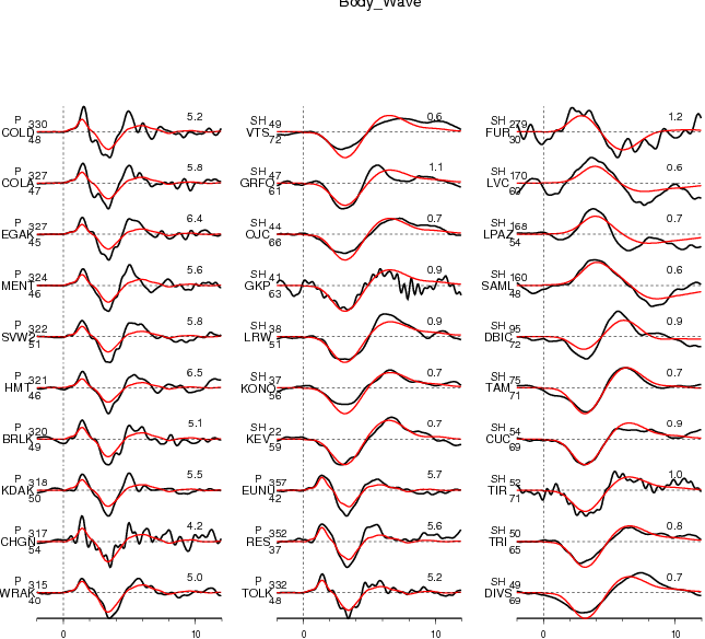
Figure 2.2. Comparison of teleseismic body waves in velocity. The data is shown in black and the synthetic seismograms are plotted in red. Both data and synthetic seismograms are aligned on the P or SH arrivals. The number at the end of each trace is the peak amplitude of the observation in micro-meter per second. The number above the beginning of each trace is the source azimuth and below is the epicentral distance.
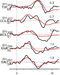
Figure 2.3. Comparison of teleseismic body waves in velocity. The data is shown in black and the synthetic seismograms are plotted in red. Both data and synthetic seismograms are aligned on the P or SH arrivals. The number at the end of each trace is the peak amplitude of the observation in micro-meter per second. The number above the beginning of each trace is the source azimuth and below is the epicentral distance.
CJ's Comments:
Not Available Yet
Slip Distribution
References
Ji, C., D.J. Wald, and D.V. Helmberger, Source description of the 1999 Hector Mine, California earthquake; Part I: Wavelet domain inversion theory and resolution analysis, Bull. Seism. Soc. Am., Vol 92, No. 4. pp. 1192-1207, 2002.
Bassin, C., Laske, G. and Masters, G., The Current Limits of Resolution for Surface Wave Tomography in North America, EOS Trans AGU, 81, F897, 2000.
Cohn, S. N., T. L. Hong, D. V. Helmberger, The Oroville earthquakes: a study of source characteristics and site effects, J. Geophys. Res., 87, 4585-4594, 1982
Acknowledgement and Contact Information
This work is supported by National Earthquake Information Center (NEIC) of United States Geological Survey. This web page is built and maintained by Dr. C. Ji at UCSB.