Preliminary Result of the Nov 14, 2007 Mw 7.81 ANTOFAGASTA, CHILE Earthquake
Chen Ji, UCSB
DATA Process and Inversion
We used the GSN broadband waveforms downloaded from the NEIC data center. We analyzed 13 teleseismic broadband P waveforms, 7 broadband SH waveforms, and 25 long period surface waves selected based upon data quality and azimuthal distribution. Waveforms are first converted to displacement by removing the instrument response and then used to constrain the slip history based on a finite fault inverse algorithm (Ji et al, 2002). We use the hypocenter of the USGS (Lat.=-22.2000 deg.; Lon.=-69.8000 deg.). The fault planes are defined using the quick moment tensor solution of the Jasha.
Result
After comparing the waveform fits based on two planes, we find that the nodal plane (strike=355.08 deg., dip=16.56 deg.) fits the data better. The seismic moment release based upon this plane is
0.667E+28 dyne.cm using a 1D crustal model interpolated from CRUST2.0 (Bassin et al., 2000).
Cross-section of slip distribution
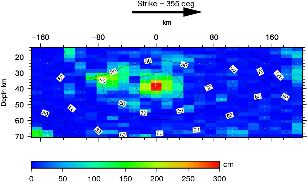
Figure 1. Cross-section of slip distribution. the strike direction of fault plane is indicated by the black arrow and the hypocenter location is denoted by the red star. The slip amplitude are showed in color and motion direction of the hanging wall relative to the footwall is indicated by white arrows. Contours show the rupture initiation time in seconds.
Comparison of data and synthetic seismograms
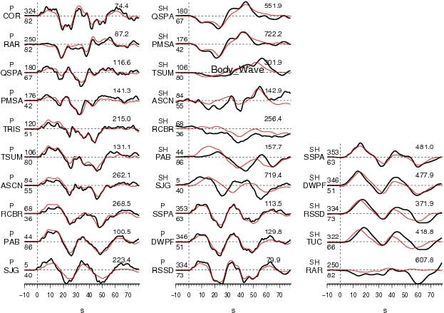
Figure 2. Comparison of teleseismic body waves. The data is shown in black and the synthetic seismograms are plotted in red. Both data and synthetic seismograms are aligned on the P or SH arrivals. The number at the end of each trace is the peak amplitude of the observation in micro-meter. The number above the beginning of each trace is the source azimuth and below is the epicentral distance.
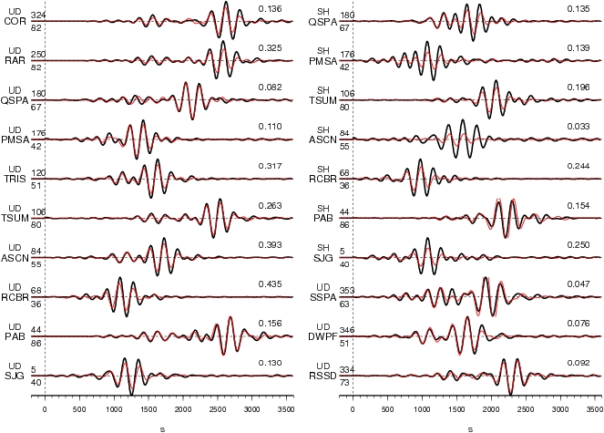
Figure 3.1. Comparison of long period surface waves. The data is shown in black and the synthetic seismograms are plotted in red. The number at the end of each trace is the peak amplitude of the observation in milli-meter. The number above the beginning of each trace is the source azimuth and below is the epicentral distance.
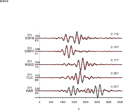
Figure 3.2. Comparison of long period surface waves. The data is shown in black and the synthetic seismograms are plotted in red. The number at the end of each trace is the peak amplitude of the observation in milli-meter. The number above the beginning of each trace is the source azimuth and below is the epicentral distance.
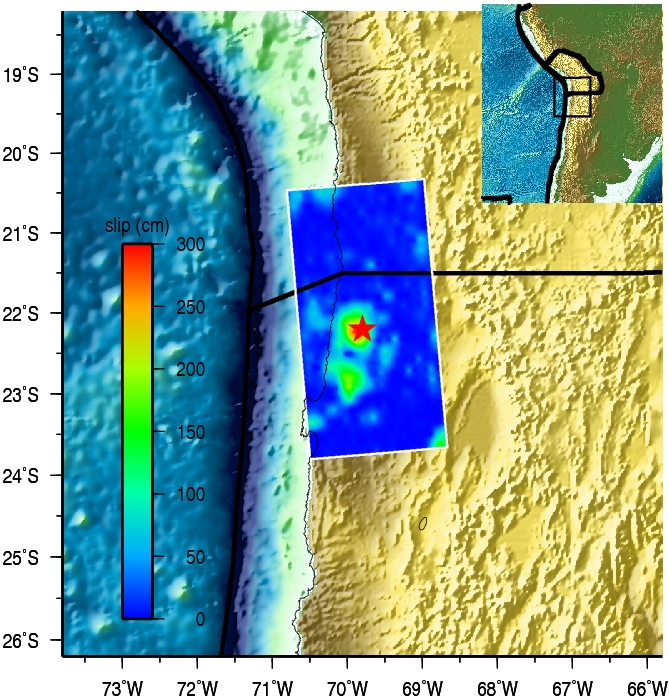
Figure 4. Surface projection of the slip distribution superimposed on ETOPO2. The black line indicates the major plate boundary [Bird, 2003].
CJ's Comments:
Not Available Yet
Slip Distribution
References
Ji, C., D.J. Wald, and D.V. Helmberger, Source description of the 1999 Hector Mine, California earthquake; Part I: Wavelet domain inversion theory and resolution analysis, Bull. Seism. Soc. Am., Vol 92, No. 4. pp. 1192-1207, 2002.
Bassin, C., Laske, G. and Masters, G., The Current Limits of Resolution for Surface Wave Tomography in North America, EOS Trans AGU, 81, F897, 2000.
Acknowledgement and Contact Information
This work is supported by National Earthquake Information Center (NEIC) of United States Geological Survey. This web page is built and maintained by Dr. C. Ji at UCSB.